Close
How can I avoid the test explosion problem?
To move from an abstract high-level scenario to concrete traffic scenarios which can be simulated, we have to define values for a large number of parameters, which is not limited to the parameters of the abstract traffic scenario. One additional aspect is the coverage of the ODD (Operational Design Domain), which describes the specific operating conditions in which the vehicle is supposed to be operated, for example, road types or even weather conditions.
So how many test scenarios will we need? If we try to simulate all parameter combinations (sometimes also called “brute force”), it will lead to an unfeasibly high amount of simulation runs. On the other hand, variation strategies which are based on random algorithms will not be able to sufficiently cover the interesting and safety-critical corner cases. So we need a smarter approach to generate test scenarios intelligently in way which still leads to a good level of confidence in the safety of the system.
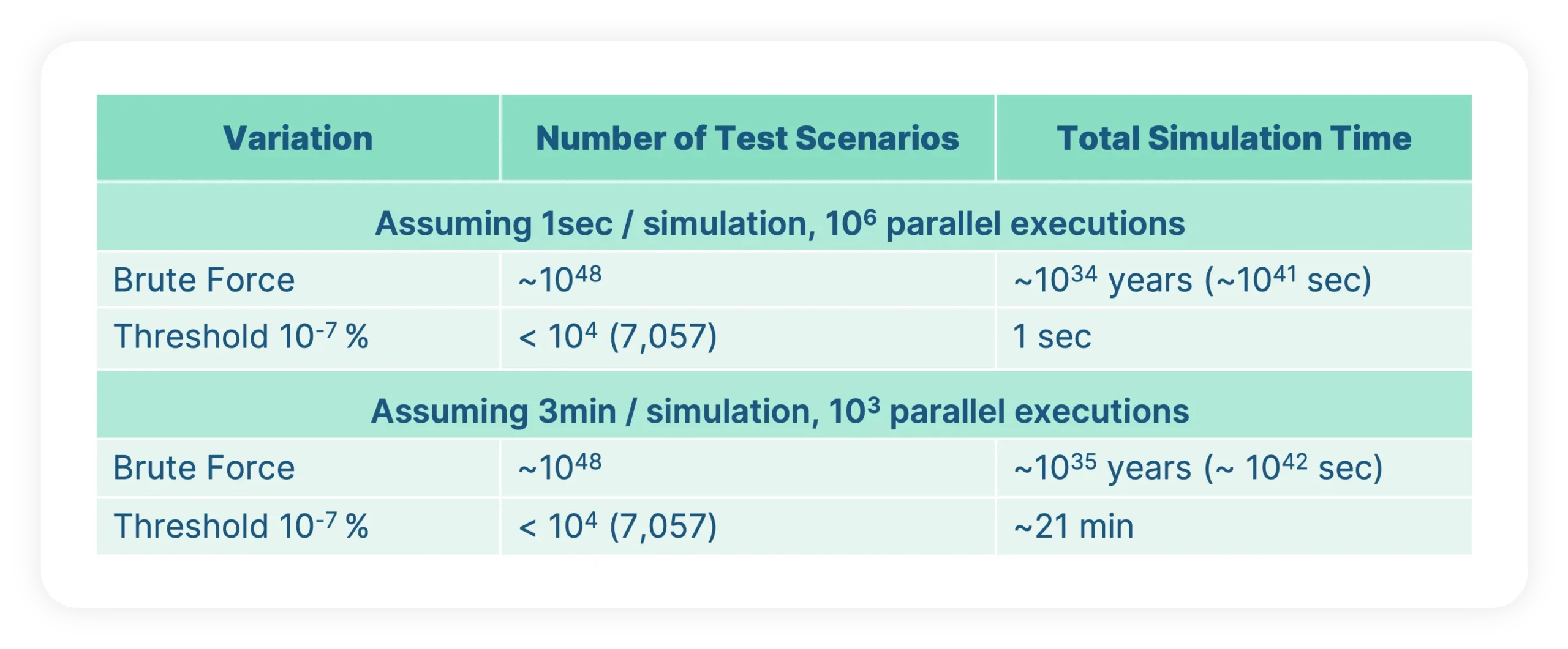
Let’s look at an example and calculate the number of test scenarios needed to cover a certain amount of parameters. If we optimistically assume only 100 parameters and only 3 different values per parameter, we will need around 10^48 (1 Octillion) test scenarios. If we then optimistically assume that each simulation takes one second, we get to an overall simulation time of 10^34 years.
Because of the complexity described above, the goal of an intelligent test scenario generation should be the following: Achieve the required confidence regarding the safety of the system without simulating all possible parameter combinations. To achieve this goal, we are reducing the number of tests by focusing on the more interesting scenarios and create less of the uninteresting ones. Of course, this immediately raises the question regarding the definition of “interesting”. In this context, the expression “interesting” can have two meanings. It can be either scenarios which are very likely to happen or scenarios which contain situations which are safety-critical. On the other hand, this means that we would have fewer test cases which are both unlikely and at the same time not safety critical. We are achieving this distribution with a two-step approach, in which each step has its own test-end criteria.
The first step separates parameter ranges into manageable parts while obeying a given variation strategy such as probabilistic distributions. This strategy enables us to get more of the likely scenarios and less of the unlikely ones. The basis for this process is the definition of multiple individual value ranges for each parameter. As an example, let’s assume a vehicle which is supposed to have a velocity between 0 km/h and 60 km/h. Similar to the concept of “Equivalence Classes” in the ISO 26262, this value range can be sliced into individual ranges, for example 0-40 km/h, 40-50 km/h and 50-60km/h. Subsequently, a probability is defined for each of these individual value ranges. For each variant of a scenario, the multiplication of these probabilities will lead to a resulting probability and a user-defined threshold allows to control which scenarios will actually get executed.
Assuming a scenario having an occurrence probability of 10% in the ODD. The scenario is varied with 100 parameters each having 3 values with the following probabilities: V1 -> 1%, V2 -> 10%, V3 -> 89%. The table below compares the number of test scenarios obtained between brute-force variation and our probability-based variation applying a threshold of 10^-7 . It shows how to efficiently reduce the number of test variants using a realistic threshold and achieving realistic simulation time.
To achieve a particularly high level of confidence regarding the behavior during safety-critical situations, the second variation step explores the parameter space using AI technology to detect SUT-specific weaknesses. The weakness will get formally defined by a weakness function that can be evaluated after each simulation run. One example for such a weakness function could be the time-to-collision, where smaller values correspond to a more safety critical situation (and therefore a higher weakness score). The weakness detection can therefore be described as an optimization problem with the goal to find local and global maxima in an n-dimensional space (n being the number of different parameters).
The outcome of this “Weakness Detection” step is either a concrete scenario leading to a critical or unwanted behavior of the SUT, or absence of weaknesses is reported in probabilistic terms.
This will lead to a lower amount of test cases for situations which are less critical (for example because all traffic participants are far away from each other) and therefore ensure that the total number of test cases does not explode.
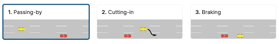
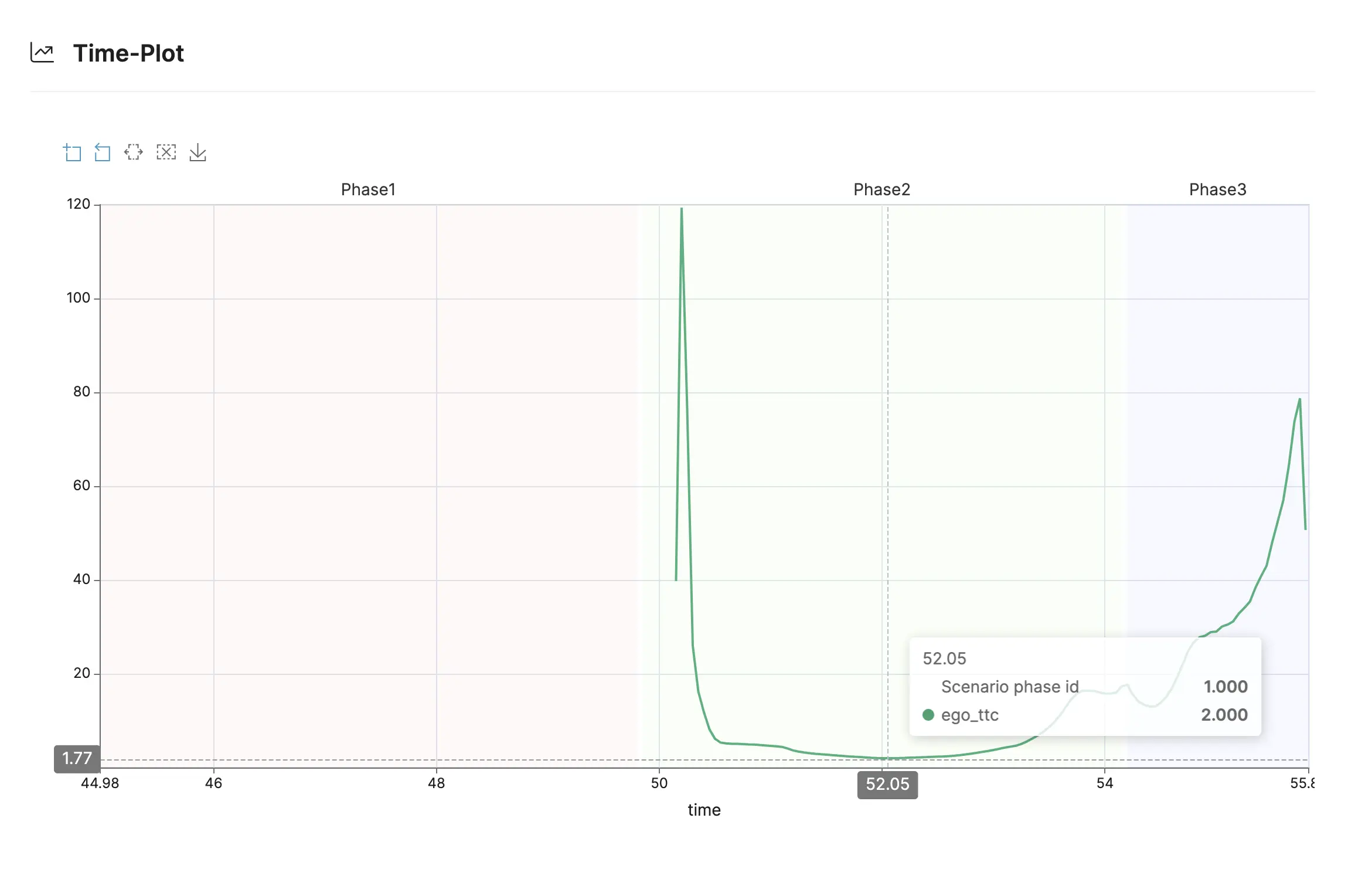
To illustrate the Weakness Detection, let’s take as example of a hazardous situation where “The minimum Time-To-Collision between the ego and a vehicle in front could fall below 2 sec”. We want to test whether the ego can prevent it or not in the context of a cut-in scenario.
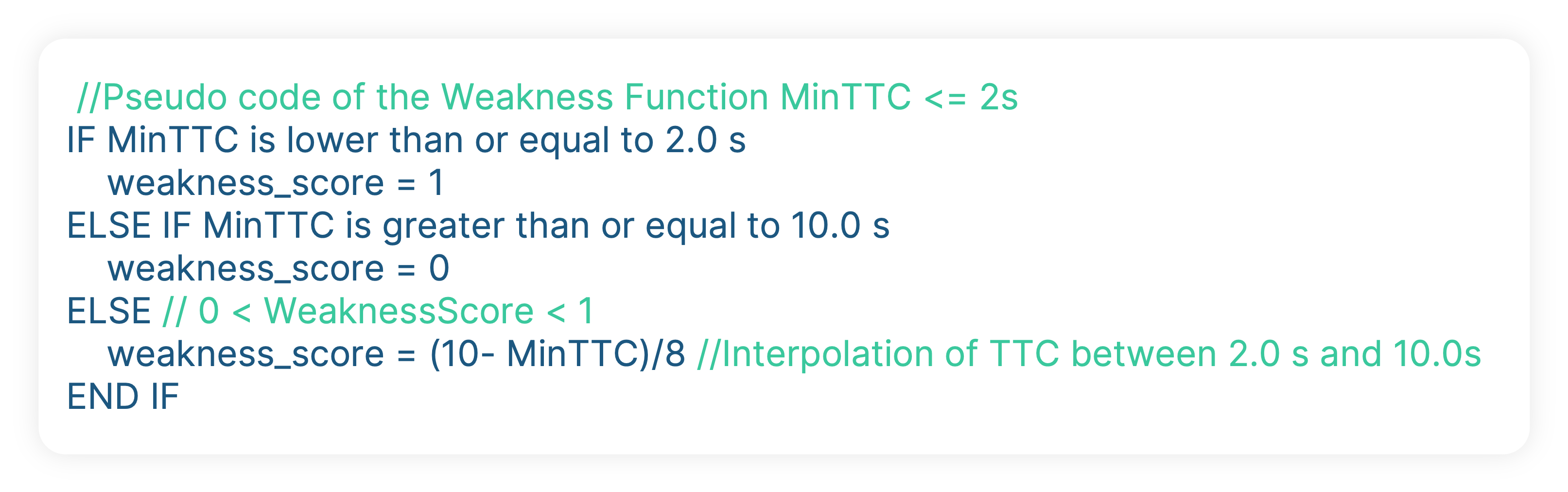
The Weakness Function: We express the hazardous situation “MinTTC <= 2s” in a function returning the score 1 when the minimum TTC is less than or equal to 2 sec and 0 if it is above 10 sec (TTC >= 10sec is considered as a sufficiently safe situation). Between 2s and 10s, the score is interpolated (See pseudo code below). While the score is less than 1, the algorithm performs further iterations exploring the parameter space until reaching the score 1. This means a scenario has been found where the MinTTC is <= 2s.
The Test Scenario: We consider a Cut-in test scenario in three phases where the following logical constraints apply:
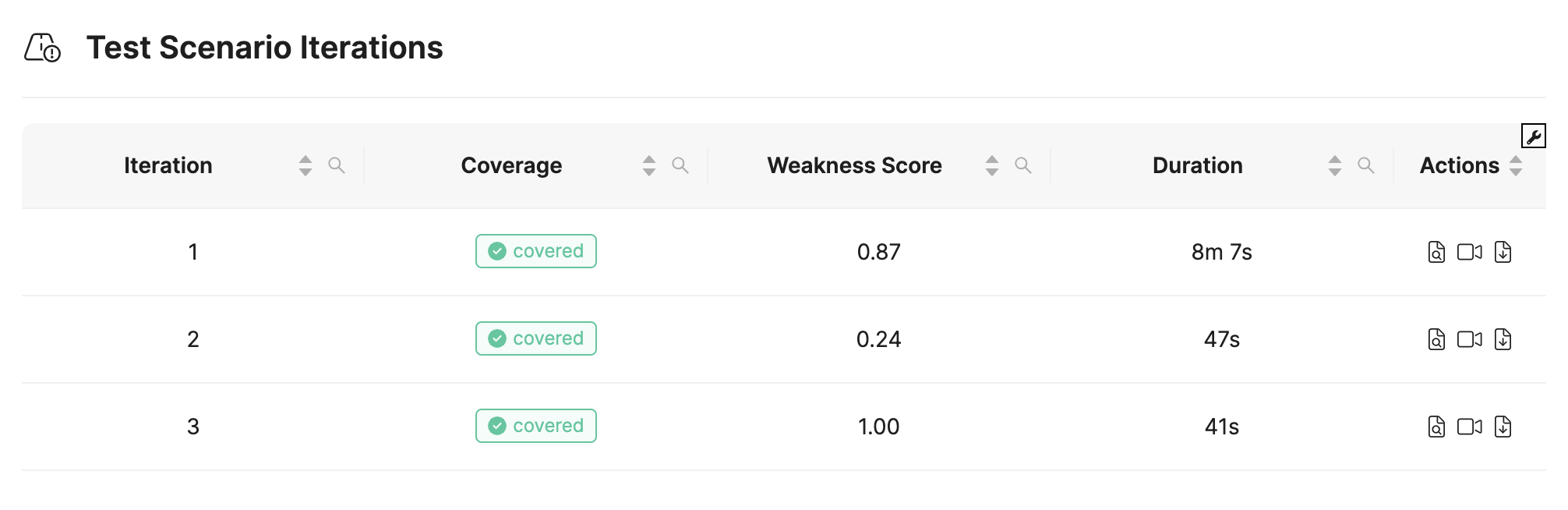
The result: When performing Weakness Detection, the analysis finds a weakness after three iterations. The weakness score reaches 1 at the third iteration and this means the algorithm has found a trajectory of the cutting-in vehicle that causes a TTC below 2 sec.


Hans Jürgen Holberg
Chief Sales Officer (CSO)
BTC Embedded Systems AG
hans.j.holberg@btc-embedded.com